- Published on
Transaction Processing or Analytics?
- Authors

- Name
- dima853
- @_dima853
Introduction to Transactions
In the early days of business data processing, writing to a database typically corresponded to a commercial transaction: selling a product 🛍️, ordering from a supplier 📦, paying employee salaries 💰, etc. Over time, the term "transaction" became established even for operations not related to money and came to mean a group of read and write operations forming a logical unit.
- 💥 Atomicity — the minimum mandatory property of any transaction
- 🛡️ Full ACID — part of reliability for critical operations
- ⚖️ In practice — different systems choose a balance between reliability (ACID) and performance (weakened guarantees)
🔄 OLTP vs OLAP: Two Different Worlds
Online Transaction Processing (OLTP) — a type of database system used in transaction-oriented applications (banks, accounting systems (ERP, CRM), booking systems, payment systems, etc.), such as many operational (core) business systems.
Two contexts where the term "transaction" is often used:
Type 1: Computer Transactions 💻
- Atomic data modification in a database
- Example:
BEGIN TRANSACTION → UPDATE → COMMIT
Type 2: Business Transactions 💰
- Economic exchange between parties
- Example: product sale, bank transfer
How they're related: OLTP uses technical transactions (type 1) to record business operations (type 2).
For example:
- 💳 Store purchase (business transaction)
- is recorded via 🖥️ SQL transaction in the database
In short: Technical transactions = tool for recording business transactions 🔧→📊
OLTP (Online Transaction Processing)
Even when databases started being used for various types of data (blog comments 📝, game actions 🎮, contacts in address books 👥, etc.), the main access model remained similar to business transaction processing.
OLTP Characteristics:
- Searching for a small number of records by key 🔑
- Inserting and updating data based on user input
- Interactive mode of operation
C Example:
// Example OLTP operation: finding customer information by ID
#include <stdio.h>
#include <string.h>

struct Customer {
    int id;
    char name[50];
    double balance;
};

struct Customer find_customer_by_id(int customer_id) {
    // In a real system, there would be a database query here
    struct Customer customer;
    customer.id = customer_id;
    strcpy(customer.name, "Ivan Ivanov");
    customer.balance = 15000.75;
    return customer;
}
OLAP (Online Analytic Processing)
Online Analytical Processing (OLAP) — an approach for quickly answering multidimensional analytical queries.
Databases also started being used for data analytics, which implies a completely different access model.
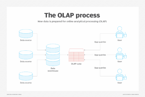
*Data Warehousing *OLAP Cube (from Online Analytical Processing) — a multidimensional data structure designed for fast and efficient analysis of large volumes of business data from various perspectives. In simple terms, an OLAP cube can be compared to a pivot table in Excel, but much more powerful and capable of working with huge amounts of information and multiple parameters (dimensions).
Let's Look at OLAP-CUBE

OLAP data is typically stored in "star" or "snowflake" schemas in a relational data warehouse or specialized data management system. Metrics are derived from records in the fact table, and dimensions are from dimension tables. but! Classic OLAP cubes (like in Microsoft Analysis Services) often store data in proprietary multidimensional formats, not in relational "star" tables. The "star" itself is the raw data storage schema on which the cube is built. Additionally, modern MPP systems (Massively Parallel Processing) like ClickHouse or Amazon Redshift often don't use cubes in the classical sense but provide similar speed for OLAP queries directly to relational tables.
🧊 OLAP Cube (Data Cube)
🎲 The term "cube" refers to a multidimensional dataset sometimes called a hypercube if the number of dimensions is more than three.
Basic Concepts:
📦 Cube — a multidimensional generalization of a two-dimensional spreadsheet
# Example: 3D data cube
dimensions = ['Products', 'Time', 'Regions']
measures = ['Sales', 'Profit', 'Budget']
Slice

Slice - the process of selecting a rectangular subset of a cube by choosing a single value for one of its dimensions, creating a new cube with one less dimension. The figure shows the slicing operation: sales metrics in all sales regions and all product categories of the company for 2005 and 2006 are "cut out" from the data cube.
Dice

Dice: The dice operation creates a subcube allowing the analyst to select specific values from multiple dimensions. The figure shows the dice operation: the new cube displays sales data for a limited number of product categories, with time and region dimensions covering the same range as before.
Drill Down/Up

Drill down/up allows the user to navigate between data levels, from the most summarized (up) to the most detailed (down). The figure shows the drill-down operation: the analyst moves from the summary category "Outdoor Protective Equipment" to sales metrics of individual products.
Roll-Up

Roll-up involves summarizing data along a dimension. The summarization rule can be an aggregate function, for example, to calculate totals along a hierarchy or apply a set of formulas such as "profit = sales - expenses". 📊💰
Computational Complexity
Common aggregate functions can be expensive to compute when rolling up: ❌
- 🐌 If they cannot be defined from the cube cells, they must be computed from the underlying data
- ⏳ Either compute them online (slowly)
- 💾 Or precompute them for possible roll-up (large volume)
✅ Efficient Aggregate Functions
Aggregate functions that can be defined from cells are known as decomposable aggregate functions and allow efficient computation.
💰 Cost of Aggregate Functions When Rolling Up
❌ Problematic Functions (expensive to compute):
📊 Median (MEDIAN)
- Requires complete data sorting for each aggregation level
- Lacks the composability property - median of subgroups ≠ median of entire group
- On-the-fly computation requires storing all original values
🎯 Percentiles (PERCENTILE)
- Similar to median, require access to the entire dataset
- 90th percentile cannot be computed from 90th percentiles of subgroups
- Must store the complete data distribution
🔢 Mode (MODE)
- Requires counting frequencies of all values
- The most frequent value in subgroups may not match the overall mode
- Requires complete recount for accurate determination
📈 Standard Deviation (STDDEV)
- Not an additive function (In the context of aggregate functions, "additivity" means the ability to compute the overall result from partial results.)
- Requires knowing the mean value and number of elements
- For accurate calculation, need ∑x and ∑x² for all data
Examples:
✅ Easily supported:
COUNT🔢MAXIMUM⬆️MINIMUM⬇️SUM➕
Because they can be computed for each OLAP cube cell and then rolled up, since the total sum (or count, etc.) is the sum of sub-sums.
❌ Difficult to support:
MEDIAN📊
Because it must be computed for each view separately: the median of a set is not the median of medians of subsets.
🔢 Mathematical Definition
(simplified) Mathematically, an OLAP cube is a projection of an RDBMS relation:
f: (X, Y, Z) → W
Where:
- X, Y, Z — cube axes (dimensions) 📐
- W — data filling each cell 💾
Projection example:
g: (Product, Time) → Sales
💾 Data Storage
OLAP data is typically stored in:
- 🌟 Star Schema
- ❄️ Snowflake Schema
- 🗄️ Specialized data management systems
Explanation (briefly)
🌟 Star Schema
- Denormalized schema
- All dimension tables linked DIRECTLY to the fact table
- Simpler and faster for queries
- Easier to understand
❄️ Snowflake Schema
- Normalized schema
- Dimension tables SPLIT into sub-tables
- More complex, but saves space
- Slower due to more JOINs
What this means in practice:
- Star → for analysis speed 📊⚡
- Snowflake → for storage economy 💾📉
Practical Examples
💼 Business Intelligence:
# Business cube dimensions:
dimensions = [
    'Products 📦',
    'Time 📅',
    'Regions 🌍',
    'Sales_Channels 🏪',
    'Customers 👥'
]

# Measures (metrics):
measures = [
    'Sales_Volume 💰',
    'Profit 📈',
    'Order_Count 🔢',
    'Average_Check 💵'
]
🏪 Retail Example:
Cube: "Store Sales"
├── Dimensions:
│   ├── Time: Year → Quarter → Month → Day
│   ├── Products: Category → Brand → Model
│   ├── Stores: Region → City → Address
│   └── Customers: Segment → Demographics
└── Measures:
    ├── Sales Amount
    ├── Quantity Sold
    ├── Profit
    └── Returns
🔗 Related Technologies
🌐 Business Intelligence:
- 📊 Data Mining — data mining
- 🏪 Data Mart — data marts
- 📈 MDX — Multidimensional Expressions
- 🔍 XML for Analysis
🛠️ Popular OLAP Systems:
- Microsoft Analysis Services
- Oracle OLAP
- Apache Kylin
- ClickHouse
💡 Key Advantages of OLAP Cube
| Advantage | Description |
|---|---|
| ⚡ Fast Response | Instant answers to complex analytical queries |
| 🔍 Multidimensionality | Data analysis from different perspectives |
| 📊 Flexibility | Interactive data exploration |
| 🎯 Intuitiveness | Visualization understandable to business users |
📋 Comparison Table: OLTP vs OLAP
OLTP is typically contrasted with Online Analytical Processing (OLAP):
| Characteristic | OLTP 🚀 | OLAP 📊 |
|---|---|---|
| Query Types | All types (read, insert, update, delete) | Mostly read-only |
| Complexity | Simple queries | Complex analytical queries |
| Volume | Large number of simple queries | Smaller number of complex queries |
| Purpose | Operation processing | Business analytics and reporting |
🏢 Data Warehousing
Why do we need a data warehouse?
Large companies can have dozens of different transaction processing systems:
- Customer websites 🌐
- Point-of-sale systems (cash registers) in stores 🏪
- Warehouse inventory tracking systems 📦
- Transportation route planning systems 🚚
- Human resources management systems 👥
Problem: OLTP systems must be highly available and process transactions with low latency. Analytical queries often require scanning large volumes of data and can interfere with transaction operations.
Solution: Data Warehouse — a separate database where analysts can run any queries without affecting OLTP operations.
🔄 ETL Process (Extract–Transform–Load)
Data enters the warehouse through the ETL process:
- Extract - data is extracted from OLTP systems
- Transform - data is transformed into a schema convenient for analysis
- Load - data is loaded into the warehouse
Real-life example: A large bank 🏦 might have separate systems for:
- Mobile banking 📱
- Credit operations 💳
- Mortgage products 🏠
- Investment services 📈
All this data is combined in a data warehouse for end-to-end analytics.
⭐ Star and ❄️ Snowflake: Schemas for Analytics
🌟 Star Schema
At the center of the schema is a fact table, surrounded by dimension tables.
Example for retail:
fact_sales(sales fact table) - at the centerdim_product(product dimension) 📦dim_store(store dimension) 🏪dim_time(time dimension) ⏰dim_customer(customer dimension) 👥
C Example:
// Structure for sales fact table
struct FactSale {
    int sale_id;
    int product_id;     // reference to dim_product
    int store_id;       // reference to dim_store
    int time_id;        // reference to dim_time
    int customer_id;    // reference to dim_customer
    double amount;
    int quantity;
    double profit;
};

// Structure for product dimension table
struct DimProduct {
    int product_id;
    char sku[20];
    char description[100];
    char brand[50];
    char category[50];
    double price;
};
❄️ Snowflake Schema
A more normalized version of the star schema where dimensions are further broken down into sub-dimensions.
Advantage of star schema: simpler for analysts!
💾 Data Warehouse Features
- Wide tables: fact tables often have more than 100 columns 📋
- Rich metadata: dimension tables contain all possible information for analysis
- Optimized for analytical queries: special storage structures and algorithms
Quick Summary: OLTP vs OLAP
🎯 Key Differences
OLTP (Online Transaction Processing)
- 💰 Real-time operation processing
- 🔄 Short transactions (read/write)
- ⚡ High availability, instant response
- 🏦 Examples: bank transfers, orders, bookings
OLAP (Online Analytical Processing)
- 📊 Analytics and reporting
- 🔍 Complex queries on big data
- 📈 Multidimensional analysis (cubes, slices, drill-down)
- 🧠 Examples: business intelligence, forecasting
🏗️ Architectural Features
OLTP
- ACID transactions 🛡️
- Normalized schemas
- Write optimization
OLAP
- Denormalized schemas (🌟 Star/❄️ Snowflake)
- Data warehouses
- ETL processes
- Read optimization
💡 What This Means in Practice
| Aspect | OLTP | OLAP |
|---|---|---|
| Purpose | Business operations 🚀 | Business analysis 📈 |
| Data | Current operations | Historical data |
| Users | Operators | Analysts |
Conclusion: OLTP ensures the company's daily operations, while OLAP helps understand trends and make strategic decisions. Both approaches are critically important but solve different problems.