- Published on
Steganography
- Authors

- Name
- dima853
- @_dima853
Steganography is the science and practice of hiding the fact that information is being transmitted, not the information itself (that's cryptography).

The same image viewed by white, blue, green, and red lights reveals different hidden numbers.
Definition
If cryptography is like sending a note in a safe that everyone sees but can't open (or in an incomprehensible language that everyone hears but doesn't understand), then steganography is like writing with invisible ink on the back of a regular postcard. The modern goal is not necessarily to achieve absolute invisibility, but to ensure that the stego-container is statistically indistinguishable from legitimate noise and doesn't attract targeted attention.
How It Works in Practice (Techniques)
The principle is always the same: hide a data container inside another, harmless carrier container without causing statistically significant anomalies.
1. In Images (Most Popular Method)
- Basic Method: Replacing Least Significant Bits (LSB).
- How it works: Each pixel's color is encoded with numbers (e.g., in RGB). Changing the least significant bit alters the color by such a small amount that the human eye won't notice.
- Example: You want to hide the letter 'A' (ASCII code 65, which is
01000001in binary) in 8 pixels. You replace the least significant bit of each pixel with one bit from the message. - Naive LSB replacement is a vulnerable and easily detectable method through statistical analysis (histogram analysis, Chi-square tests). Modern adaptive methods (e.g., syndrome coding, spreading across multiple bit planes) actively combat anomalies. Basic LSB is used only for Proof-of-Concept or against incompetent adversaries.
1) Histogram Analysis
- What it is: A graphical representation of the distribution of values (e.g., pixel colors in an image).
- Purpose in steganalysis: To detect statistical anomalies that arise after data embedding.
- How it works:
- A "clean" image has a smooth, continuous histogram.
- Naive LSB method creates characteristic "steps" or paired values in the histogram because when replacing the least significant bit, pairs of values (0 and 1, 2 and 3, etc.) become almost equally probable. This is easily noticeable visually on a graph.
2) Chi-square Test (χ²)

Chi-squared distribution, showing χ2 on the first axis and p-value (right tail probability) on the second axis.
1. What is k (Degrees of Freedom)
In simple terms: k is a parameter that indicates the "complexity" or "dimensionality" of our analysis.
In the context of steganalysis (LSB checking):
- Imagine we're analyzing an image's histogram.
- We look at pairs of values (0 and 1, 2 and 3, 4 and 5, etc.) that might have aligned due to LSB replacement.
kis the number of such pairs we're checking.- The larger
k, the more data we're analyzing.
On the graph: Each line (k=1, k=2, etc.) is a separate Chi-square distribution for a different number of degrees of freedom. Notice that as k increases, the curve "flattens" and shifts to the right. (need to look "from the side of zero" (left to right))
2. What is p-value (Probability / Significance Level)
In simple terms: p-value is the probability that the result we observed (alignment of pairs in the histogram) occurred by chance.
In the context of steganalysis:
- High
p-value(close to 1): High probability that the histogram looks like this simply by chance. Conclusion: Steganography is likely NOT present. - Low
p-value(close to 0): It's extremely unlikely that such perfect alignment of pairs happened by chance. Conclusion: The file likely contains hidden data embedded using the LSB method.
On the graph: p-value is shown on the vertical axis as "right tail probability". When our calculated Χ² value falls far into the right "tail" of the distribution (shaded area), the p-value becomes very small. (p-value is determined by the horizontal axis (X²) from right to left, not by the vertical axis)
Simply put:
- Histogram analysis is "look at the graph and see suspicious patterns".
- Chi-square test is "calculate and get a number proving the file is suspicious".
3) Syndrome Coding
- Essence: This is not a data embedding method, but a matching method. It allows embedding a message without changing some bits of the carrier.
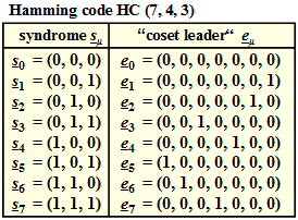
Left Column: Syndromes (S)
These are all possible syndromes (3-bit checksums) that can be computed from a 7-bit block.
Right Column: "Coset Leaders" (e)
These are minimum weight error vectors (with the minimum number of ones) corresponding to each syndrome.
Note: Each vector e contains only one one - this is the minimal possible change!
The table shows the minimal impact needed to obtain the desired "fingerprint" (syndrome).
How This Works in Steganography (briefly):
STEP 1: Preparation
- We have a cover block (7 bits from the image):
C - We have a message (3 bits) we want to hide:
M
STEP 2: Compute syndrome of the cover block
- Compute the syndrome of the cover block:
S_cover = H × C(where H is the parity-check matrix) - In the table, this corresponds to finding the syndrome
S_cover
STEP 3: Compare syndromes
- If
S_cover = M→ Already matches! Change nothing. Usee0 = (0,0,0,0,0,0,0) - If
S_cover ≠ M→ Need to find an error vectoreto change the syndrome
STEP 4: Find error vector
- Look in the table for a syndrome
Sequal to our target messageM - Take the corresponding coset leader
e
STEP 5: Embedding
- Modify the cover block:
C_stego = C + e - Now the syndrome of the new block:
S_stego = H × (C + e) = H×C + H×e = S_cover + S = M
- Advantage: Drastically reduces the number of carrier modifications. Ideally, only 1 bit per block is changed, making attacks based on LSB replacement statistics practically useless.
Spreading Across Multiple Bit Planes
- Essence: Abandoning the naive approach where data is hidden only in the 1st least significant bit (LSB). Instead, the message is "spread" across several least significant bit planes.
- How it works:
- A pixel image can be represented as a "stack" of bit planes: from the most significant to the least significant.
- Naive LSB uses only the bottommost plane.
- Modern methods (e.g., HOLMES) embed data simultaneously into the 1st, 2nd, and sometimes 3rd bit planes, adapting the embedding depth to the image texture.
- In complex textures (noise, grass), even higher-order bits can be changed, as the eye won't notice. In smooth areas (sky) — only the least significant ones.
- Advantage: Drastically increases capacity and, more importantly, resistance to steganalysis. Statistical anomalies arising from replacing only the 1st LSB are blurred and become indistinguishable from the image's natural noise.
Bit Planes
Basic Concept
A bit plane of a digital discrete signal (such as an image or sound) is a set of bits corresponding to a specific bit position in each of the binary numbers representing the signal.
Simple example: For 16-bit data representation, there are 16 bit planes:
- The first bit plane contains the set of most significant bits (MSB)
- The sixteenth contains the least significant bits (LSB)

The 8 bit-planes of a gray-scale image (the one on left). There are eight because the original image uses eight bits per pixel.
Significance of Bit Planes
It can be observed that:
- The first bit plane gives the coarsest but most critical approximation of the medium's values
- The higher the number of the bit plane, the less its contribution to the final result
Thus, adding each subsequent bit plane gives a better approximation to the original value.
Mathematical Contribution of Bit Planes
If a bit in the n-th bit plane in an m-bit dataset is set to 1, it contributes a value of 2^(m−n), otherwise it contributes nothing. Therefore, bit planes can contribute half the value of the previous bit plane.
Example with the 8-bit value 10110101 (181 in decimal):
| Bit Plane | Value | Contribution | Cumulative Total |
|---|---|---|---|
| 1st | 1 | 1 × 2⁷ = 128 | 128 |
| 2nd | 0 | 0 × 2⁶ = 0 | 128 |
| 3rd | 1 | 1 × 2⁵ = 32 | 160 |
| 4th | 1 | 1 × 2⁴ = 16 | 176 |
| 5th | 0 | 0 × 2³ = 0 | 176 |
| 6th | 1 | 1 × 2² = 4 | 180 |
| 7th | 0 | 0 × 2¹ = 0 | 180 |
| 8th | 1 | 1 × 2⁰ = 1 | 181 |
Technical Note
The term "bit plane" is sometimes used as a synonym for "bitmap", however technically:
- The former refers to the location of data in memory
- The latter refers to the data itself
Noise Analysis in Bit Planes
One aspect of using bit planes is determining whether a bit plane is random noise or contains meaningful information.
Calculation method: Compare each pixel (X, Y) with three neighboring pixels:
- (X − 1, Y)
- (X, Y − 1)
- (X − 1, Y − 1)
If a pixel matches at least two of the three neighboring pixels, it is not considered noise.
Criterion: A noisy bit plane will have between 49% to 51% of pixels that are noise.
Applications of Bit Planes
1) Media File Formats
Using PCM audio as an example:
- The first bit in a sample denotes the sign of the function (determines half of the entire amplitude range)
- The last bit determines the exact value
Important principle:
- Changing more significant bits leads to greater distortion
- Changing less significant bits is less critical
In lossy media compression using bit planes, this allows more freedom for encoding less significant bit planes, while more significant ones must be preserved as accurately as possible.
Pulse Code Modulation (PCM)
Pulse-code modulation (PCM) is used to digitize analog signals. Virtually all types of analog data (video, audio (voice, music), telemetry) allow the use of PCM.
PCM is like "digitizing" sound or any other analog signal for use in the digital world. Without PCM, we couldn't store music on computers or transmit voice over the internet.

Example of 4-bit (16-level) PCM. Shows quantization of an analog signal and bursts of impulses encoding the samples. Transmission in the channel is performed with the most significant bits first.
Modulation
Example of 4-bit (16-level) PCM. Shows quantization of an analog signal and bursts of impulses encoding the samples. Transmission in the channel is performed with the most significant bits first.
PCM Operating Principle
In pulse-code modulation, the analog transmitted signal is converted into digital form through three operations:
- Time sampling (measuring the analog signal at equal time intervals (obtaining samples))
- Amplitude quantization (rounding each sample to the nearest level from a finite set of values)
- Encoding
Converting Analog Signal to Digital
An analog-to-digital converter (ADC) is used to convert an analog signal to digital. The ADC measures the amplitude of the analog signal at equal intervals - obtains instantaneous values or signal samples, then converts the samples into binary words.
The measured instantaneous value (sample) of the analog signal is quantized by levels (rounded to the nearest integer). The number of quantization levels is usually equal to or a multiple of an integer power of 2, for example:
- 2³ = 8 levels
- 2⁴ = 16 levels
- 2⁵ = 32 levels
The level number is encoded with binary words of length 3, 4, 5, etc. bits.
Forming Signal for Transmission
Then the ADC's output words in parallel code are encoded by feeding them to a shift register clocked by an auxiliary shift generator. At the output of the shift register, bursts of encoded impulses in serial code are formed. Then the impulse bursts are transmitted into the communication channel.
Note: An impulse burst is periodically repeating impulses over a fixed time interval.
Sampling Frequency
The signal sampling frequency (or digitization rate, sampling frequency) to avoid information loss, according to the Nyquist–Shannon sampling theorem, must be at least twice the maximum frequency in the analog signal's spectrum.
Technical Implementation
There are specialized integrated circuits designed for PCM, combining ADC, shift register, clock generators, and other devices.
Demodulation
A demodulator is installed at the receiving end of the communication channel. In the demodulator, impulse bursts are fed to the serial input of a shift register. After shifting all bits of the impulse burst into the shift register, the word from the shift register in parallel code is written to the input register of a digital-to-analog converter (DAC).
The DAC converts the encoded samples of the transmitted analog signal back into analog form. A stepped analog signal is formed at the DAC output. Smoothing of the steps is performed by a low-pass filter (LPF), at the output of which the transmitted analog signal is formed. The LPF cutoff frequency is chosen to be less than or equal to twice the sampling frequency.
Digital Codes in PCM
A wide variety of binary codes are used to encode samples in PCM:
- Ordinary representation of numbers in the binary numeral system, with sequential transmission of bits of the binary number can be done either least significant bits first or most significant bits first
- Various codes with error detection and correction in the transmission channel, for example, Hamming code, Reed–Solomon code, etc. The simplest of them is a redundant code with parity bit transmission
- Codes that eliminate the DC component in the encoded two-level impulse signal, for example, self-synchronizing Manchester code
PCM Variants
Differential Pulse-Code Modulation (DPCM)
PCM combined with delta encoding, where the signal is encoded as the difference between the current and previous measured values. For audio data, this modulation method reduces the required number of bits per sample by about 25%.
Adaptive DPCM (ADPCM) — a variant of DPCM with variable quantization step size. Changing the step size allows reducing bandwidth requirements for a given signal-to-noise ratio.
LPCM (Linear pulse code modulation)
Linear pulse-code modulation.
Practical Application
- In digital and IP telephony, PCM is used to convert voice audio signals into a digital stream transmitted at 64 kbit/s (primary digital channel)
- PCM is used to convert analog audio signals to digital for storing signals on digital devices and media (digital audio recording). File formats: WAV, MP3, WMA, OGG, FLAC, APE
- PCM was previously used in modem communication protocols ITU V.90 (only incoming signal to the client) and V.92 (incoming and outgoing signal) to provide a maximum connection speed of 56 kbit/s
2) Raster Displays
Some computers displayed graphics in bit plane format, specifically:
- PCs with EGA video cards
- Amiga
- Atari ST
This contrasted with the more common packed format. This organization allowed performing certain classes of image operations using bitwise operations (especially with the blitter chip), as well as creating parallax scrolling effects.
3) Motion Estimation in Video
Some motion estimation algorithms can be performed using bit planes (e.g., after applying a filter to convert salient edge features into binary values).
This can sometimes provide a good enough approximation for correlation operations with minimal computational cost. This method is based on the observation that spatial information is more significant than actual values.
Technical detail: Convolutions can be reduced to bit shift and popcount operations, or performed in specialized hardware.
4) Neural Networks
Bit plane formats can be used to feed images into:
- Spiking neural networks
- Neural networks/convolutional neural networks with low-precision approximations
5) Software
Many image processing packages can split an image into bit planes. Open-source tools include:
Pamarithfrom the Netpbm packageConvertfrom ImageMagick
2. In Audio and Video
- Same principle: Making changes imperceptible to human hearing/vision in the audio track (masking in critical hearing bands, modifying phase spectrum) or in video frames. For example, adding quiet echo signals with specific delays that encode information.
3. In Text
- Methods: Changing the number of spaces or tabs (difficult to detect visually but trivially revealed by analyzing source code), using invisible Unicode characters (Zero-Width Joiner, Zero-Width Non-Joiner), algorithmic synonymization.
- Most primitive historical example: Pricking specific letters in text with a pin that form a secret message.
4. In Network Traffic (Network Steganography)
- Methods: Hiding data in service fields of network packet headers (e.g., in IP ID, TTL field, or flags), in the time delay between packets (timing channels), or in "empty" TCP segments.
- This is especially dangerous because detecting such traffic with standard protection tools (firewalls, IDS) is almost impossible, especially inside an encrypted channel (HTTPS), which hides the stego-carrier itself from deep packet inspection.
Steganography vs Cryptography
| Parameter | Cryptography | Steganography |
|---|---|---|
| Main Goal | Hide the CONTENT of the message | Hide the VERY FACT of the message's existence |
| If Discovered | Enemy knows about the existence of a secret message. Its content (hopefully) is protected. | COMPLETE FAILURE. The very concept of secrecy is destroyed. |
| Attention | Can attract attention (encrypted correspondence is suspicious by itself) | Avoids attention (looks like normal traffic) |
| Protection | Mathematical strength of algorithms and key length | Statistical indistinguishability from the original carrier and resistance to steganalysis |
Important conclusion: In serious systems, they are combined. First, the message is encrypted (cryptography), then hidden in a carrier (steganography). This way, even if the enemy discovers the hidden data, they cannot read it.
Real Threats and Applications
1. Cyber Espionage and APT Attacks
- How it's used: Malware steals data and exfiltrates it, disguising it as normal traffic. Common scheme: data is hidden in an image uploaded to a public resource (forum, GitHub, cloud), and the malware on the compromised machine downloads it. Encrypted HTTPS connection hides the stego-carrier from inspection.
2. Circumventing Censorship in Totalitarian Regimes
- How it's used: Activists and journalists use steganography to transmit information through blocked channels without attracting the attention of censors who look for keywords in plain text.
3. Concealing Criminal Activity
- How it's used: Criminal communities exchange instructions and data by hiding them in files posted on public forums and cloud storage. Important clarification: using social media is problematic as they often recompress images, destroying the stego-container.
4. Digital Watermarks (the other side)
- This is a legal application: Copyright holders embed invisible marks into their content to confirm authorship and track leaks. This is steganography where the goal is not to hide the fact of transmission, but to hide the mark itself until the moment of verification.
Detection (Steganalysis)
Steganalysis is the art of detecting steganography.
- Methods: Statistical analysis of the carrier file for anomalies (histogram analysis, Chi-square tests), entropy analysis, searching for traces of specific steganography tools, machine learning to identify patterns.
- Hard truth: A universal detector does not exist. Detection is difficult and often impossible without a hypothesis about the method used. However, against specific, known methods (like naive LSB), steganalysis can be highly effective. Channel capacity is low, but it's sufficient for transmitting keys, passwords, or control commands.
Final Verdict
Steganography is a powerful, dangerous, and often underestimated tool. In the cybersecurity arsenal, it represents a persistent and hard-to-detect threat because an attack based on it is practically invisible against the background of legitimate traffic. This is not a "zero-day vulnerability", but a fundamental technique leading to an eternal battle between concealment and detection methods. For an infosec specialist, understanding steganography is not an option but a necessity, especially during incident investigation and defense against targeted attacks.